


Instructions
Shown below is a selection of software tools developed for the beamline. These apps are all written in Python, hence should work on any platform (Linux, Mac, Windows).
For those using Windows, it helps to set up a python environment with the required packages. One suggestion is to use Anaconda Navigator.
Here are some instructions:
# Create a clean environment in Anaconda Navigator. Install the default
# Python version. I currently use Python v3.9.x. Experiment with the latest # version(s) at your own risk.


# For the freshly created environment, open a terminal and install the
# dependencies by running:

pip install -r requirements.txt

# You can now start the app in the script directory by running:

python 'filename'.py


# ADVANCED INSTALLATION: If you want to regenerate the provided
 # 'requirements.txt' file , install:

pip install pipreqs

# ...and run:

pipreqs . --force


# If you want to use the shortcut, please edit the .bat file!
Menu
ED-XRD
- Detector calibration coefficients
- 2Θ calculator
- File conversion
- NXS Frameviewer & exporter
- EoS crossfit utility
- Stress (lattice strain) calculator
- PDIndexer troubleshooting
- GSAS-II Guide and troubleshooting
- GSAS-II lst file export (cell params and density)
LVP
Acoustic Emission
ED-XRD
I. Detector calibration between channel and energy
This tool will fit all the peaks produced by the radionuclides Ba133 and Co57 and calibrate a linear and quadratic relationship between channel and energy. You can only use the nxs files obtained at beamline station P61B. This is the first required step when starting a beam time. This tool also produces an input (txt) file for the app NXS2GSAS.
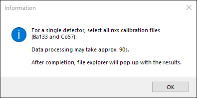
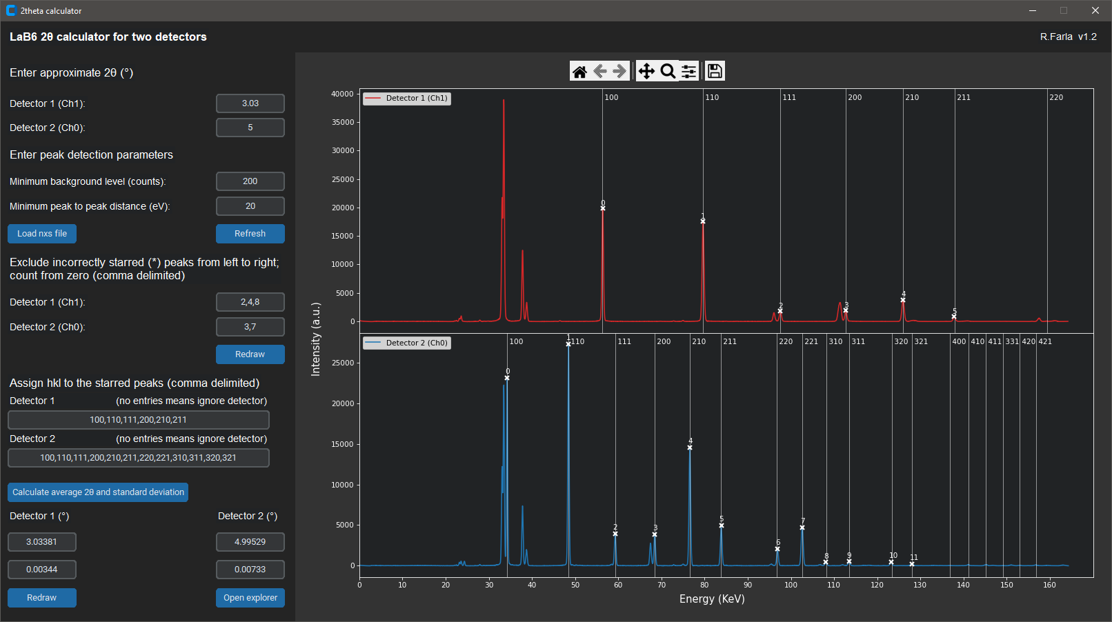
II. 2Θ calculator
A new software tool was developed to obtain the detector positions (2theta) by fitting LaB6. This should be done at the start of a beam time. Please run it in a dedicated Anaconda python environment.
The beamline station P61B uses the NIST LaB6 660c standard with a calibrated lattice parameter of a = 0.415 682 6 ± 0.000 008 nm (95% confidence) to precisely estimate the diffraction angles the detectors are positioned at.
(!) If you require measurements using a different NIST standard (e.g. Si), please discuss with the beamline staff well in advance of your beam time. If you have such a standard material, we request you to bring it along.
Update! v1.3. It is now possible to load an nxs file containing only 1 channel (e.g. if only 1 Ge-detector was used). In addition, for all peaks fitted with the pseudo-Voigt function, an additional txt file is generated containing the full output of the peak fitting, including Chi-squared reduction values. Plus minor bug fixes.
III. File conversion
The file format of the diffraction data saved by the Tango device of the digital analyser for the Ge-detectors is HDF. The file extension is nxs. Below are two tools to convert the diffraction data to readable formats for futher analysis (outside PDindexer).
The first app outputs channel and intensity in two column csv format, without a channel to energy conversion.
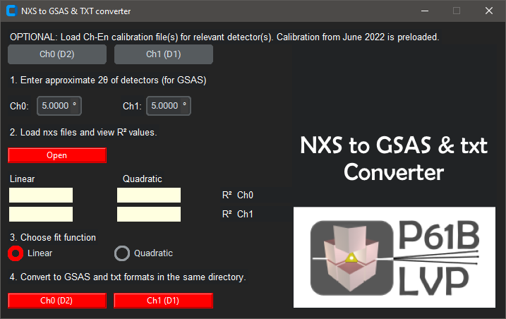
The second app NXS2GSAS converts the NXS file to GSAS format for each detector/channel to be used for refinement in GSAS and GSAS-II (since Jan 2022). Additionally, the app writes 2-column txt files for energy and intensity.
-> UPDATE 29.04.2022 - NSX2GSAS no longer requires you to load the channel to energy calibration files. The latest calibration (April 2022) is now included in the script.
As GSAS-II now supports ED-XRD, you can download and install it normally. The converted nxs to GSAS files are compatible. When you import GSAS data to GSAS-II, you must also import an instrument calibration file (see GSAS-II Guide and troubleshooting.
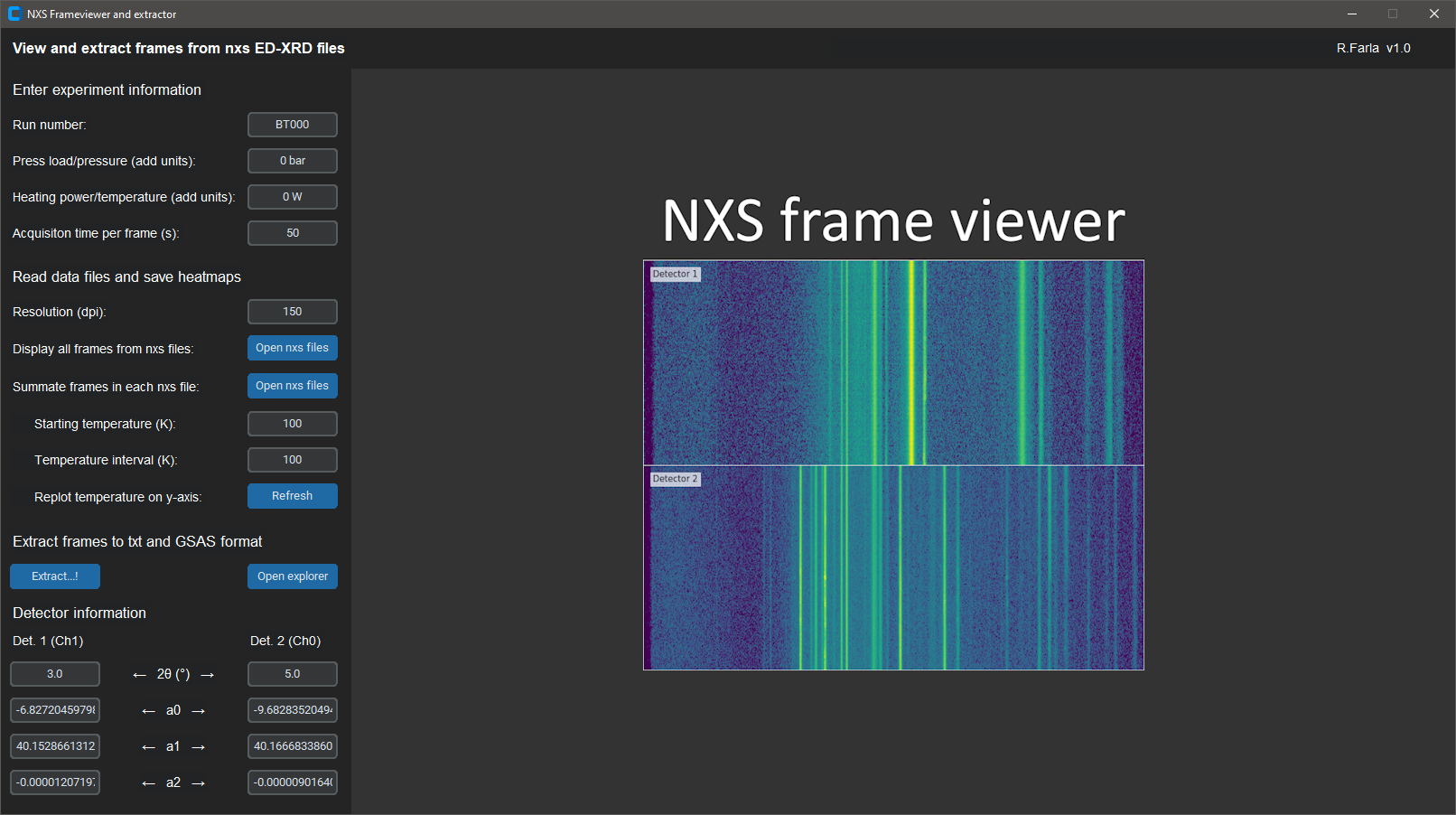
IV. NXS Frameviewer & exporter
This application will help you view large amounts of (ED) diffraction data in a heatmap using the scientifically-accepted colourmap called 'viridis' (see Matplotlib documentation). The displayed data are not modified in any way except by a channel-energy conversion. This is just an alternative presentation of stacked ED-XRD spectra.
The app offers several benefits.
1) Routinely, you can collect a diffraction pattern up to 50 s duration. However, it is also possible to collect data every second for 50 frames. In software, such as PDIndexer, you cannot see the difference because it summates all the frames when loading the nxs file. With this app, you can view each frame as a fucntion of collection time, stacked in a heatmap. You can also open multiple nxs files with each many frames and view them all in a stack.
2) The app can also summate all the frames in multiple nxs files before viewing a stacked sequence. This is very useful if you need good resolution/intensity to see and track the peak positions. You can also observe peak shifts due to deviatoric stress (lattice microstrain) with the detectors in the deformation geometry.
3) You can convert the time scale on the y-axis to temperature if you want to show the evolution of peaks during heating (at regular intervals).
4) You can extract each frame as separate data files in GSAS-II and txt format for point 1 above. Furthermore, you can also do this for point 2 above. Essentially, this is the same as using the NXS2GSAS app, above.
5) The app saves a high-resolution png image of the heat maps when loading the data (you can decide on the dpi quality). NB. due to the dark GUI settings of the app, the saved maps have a black background unfortunately. For use in publications, use any image-editing software (eg. Paint.net) to invert the background to white, with black text. Just make sure to first create selection rectangles of the data area and colour bar, invert this selection, and then invert the image background.
(!) In the app, make sure to update the quadratic equation parameters after a channel-energy calibration of both detectors.
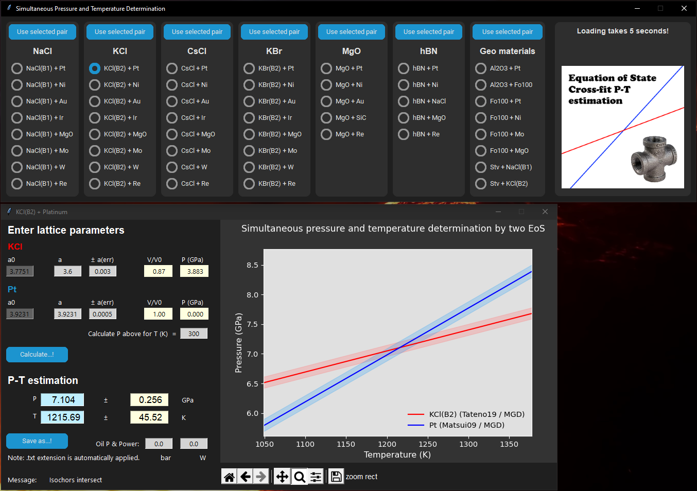
V. EoS Crossfit utility
This tool is very useful to estimate pressure and temperature in situ simultaneously without a thermocouple, via XRD and the equation of state (EoS) of two (or multiple pairs of) materials in the cell assembly. Note, it is best if both materials are in a mixture with suitable proportions. See below for more info. The starting grain size of the powders should be around 1 micron.
Mixing powders of 2 materials. Obtain the Reference Intensity Ratios (RIR) of both materials (e.g. from Match! or some other crystallography software). Divide them by each other to obtain the mixing ratio.
The tool uses Burnman for the calculations and mineral database. Please cite my paper: Farla 2023 and Burnman.
See installation instructions on the official DESY Gitlab website. Link below.
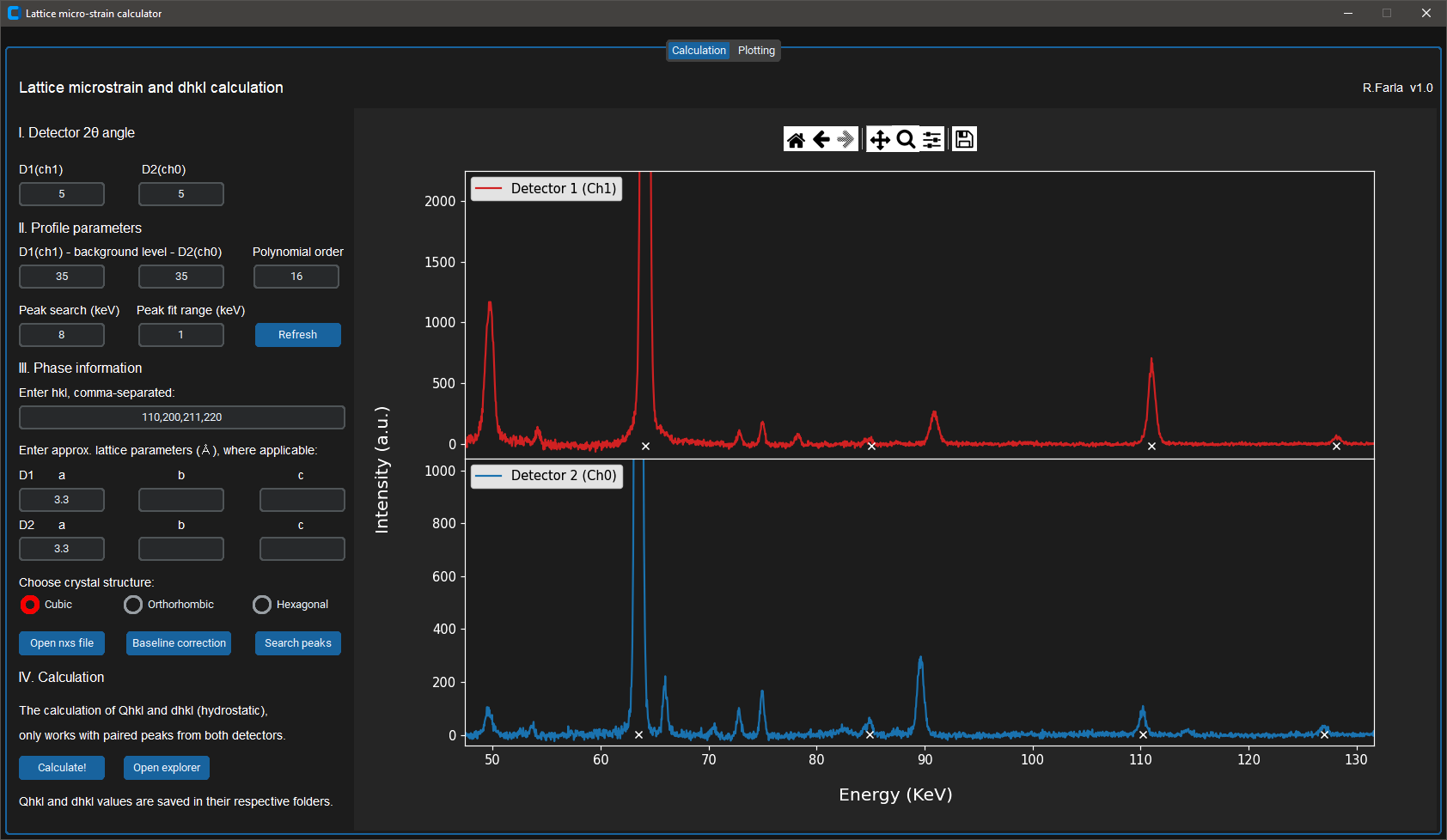
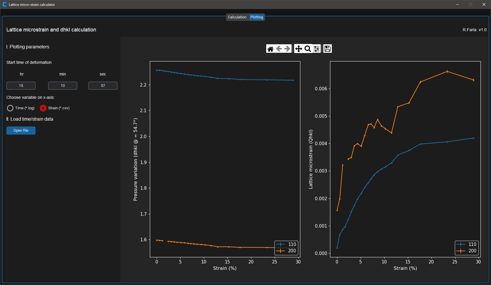
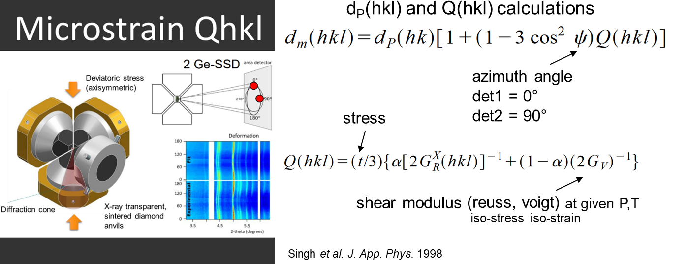
V. Stress (lattice strain) calculator
This application is useful for deformation experiments on cylindrical samples in the Aster-15 LVP. Use it to process diffraction data from two detectors to calculate the lattice microstrain Q(hkl) and the hydrostatic pressure dP(hkl) on any sample with cubic, orthorhomic or hexagonal crystal structure.
The calculation only works if one detector is at an azimuthal position (solid angle) of 0 degrees and the other detector at 90 degrees, and the same peaks can be indexed.
VII. PDIndexer troubleshooting
First, download the latest version of PDIndexer here: PDIndexer
You also need the latest version of Microsoft .NET 7.0 runtime: dotNET 7.0 runtime
And you also need a recent version of the HDF5 libraries: HDF5 pre-built binaries
Simply install these above and PDIndexer should load.
- PDIndexer does not require administrative priviliges, it will install in the /user directory.
- You must use regional settings in MS Windows where the decimal point is used (e.g. UK), rather than the comma (as is common in Germany).
- After an update, I STRONGLY recommend to reset the crystals (File -> Revert crystals to the initial state) and clear the registry (Option -> Clear Registry (check and restart)).
In case you do not have any EDXRD data from P61B yet, you can load a dummy datafile:
Download datafile
You will also need the channel to energy calibrations before you can open any data files (.nxs). Below are the calibrations from May 2023.
CH0 (detector 2)
- a0: -27.704634233000
- a1: 40.190729052025
- a2: -0.000014869539
- a0: -0.221663132172
- a1: 40.158842651421
- a2: -0.000014072325
VIII. GSAS-II Guide and troubleshooting
We recommend you to refine your ED-XRD data using GSAS-II in order to obtain the unit cell volume and density of the phases at high PT conditions in the LVP. You can download a guide on how to do this.
From GSAS-II version 5625 (and latest version), both Gaussian and Lorentzian parameters can be included in the peak fitting. This is particularly useful if more than one phase is present and they have very different peak shapes. For the latest versions you need a different instrument parameters file when importing ED-XRD powder data than when using the old version with only Gaussian parameters. You can download examples of these instrument parameter files below.
Note that data collected in your beam time cannot use these files directly. They have to be generated from the refinement of ED-XRD data of the NIST standard LaB6 collected from both Ge-detectors at particular diffraction angles (2theta). This can be done at the start of your beam time, or any time later using the raw (nxs to GSAS converted) data files of LaB6.
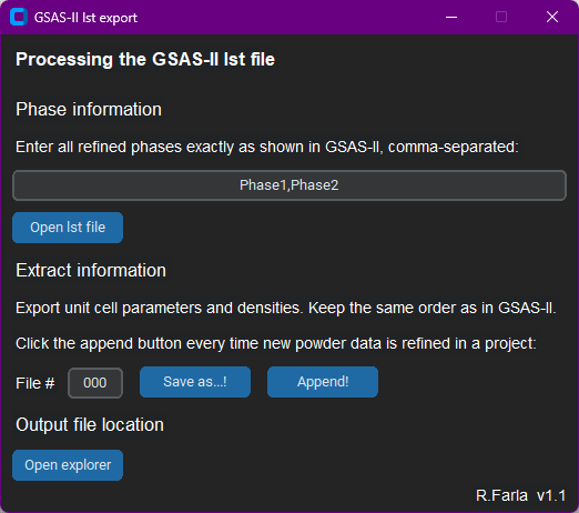
IX. GSAS-II lst file export (cell params and density)
This utility is useful for quickly extracting the unit cell parameters and density of all phases from the GSAS-II lst file saved after each refinement. It is most effective when you created a GSAS-II project with multiple imported powder data. The lst file generated by GSAS-II takes the filename of the project, so each time you refine an ED-XRD pattern, the refined unit cell parameters and density of each phase are overwritten in this file. Use the app to extract this information from the lst file between refinements of the powder data in the GSAS-II project and append each result into a txt file (leave the app open). The txt file can be edited e.g. using MS Excel to plot the data, or can be used for further data processing (e.g. to fit an EoS to the PVT data of the phase).
LVP
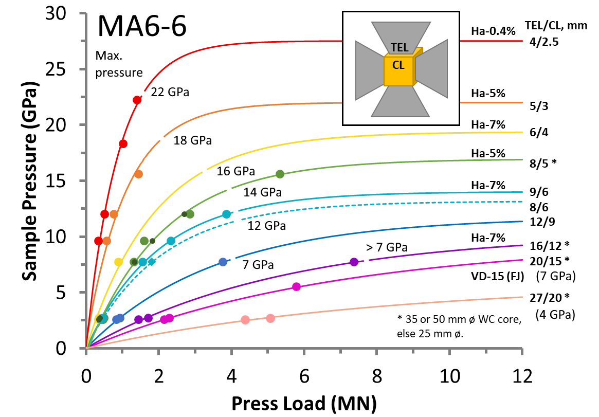
I. Sample pressure calculator
The calculators are based on these pressure calibrations:

II. Aster-15 Logviewer (MATLAB)
If you want to quickly and interactively visualize the press log data saved by the Aster-15 LVP, as well as the logged heating data if the AC heating system was used, then you can run this MATLAB script.
Now you can also download the executable for the Aster-15 logviewer, below. To run it, you also need to download and install the correct MATLAB runtime version 9.12 (R2022a). You can get it from here.
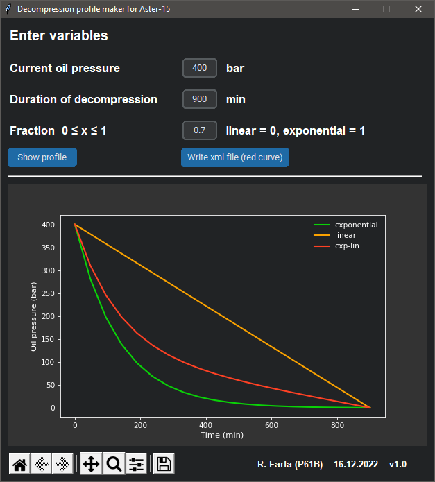
III. Decompression profile maker for Aster-15
There are cases where a linear decompression curve is not ideal. For example, it could lead to a decompression blow out or the sample will be under tension, causing cracking. This app will generate an exponential decay curve for decompression and you have the option to change the shape between a linear and purely exponential function. This curve can be saved to an xml file, which can be imported into the Aster-15 LVP software. The software accepts up to 19 steps in the pressure profile.
Extract the zip file, and execute 'profilemaker.exe'
Acoustic Emission
I. Extraction of AE data (Mistras DTA file)
For Acoustic Emissions detection experiments in the LVP, the Mistras/GMA acquisition software AEwin is used. It is now possible to extract your AE data from the proprietary file format *.dta by using MistrasDTA:
Using the above tool, I created a script and packaged an executable to extract the waveforms of events and their AE characteristics. You can download both below:
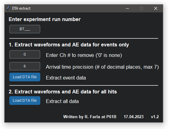
Version 1.2: Correction applied the precision on the time of arrival (TOA) of the hits/events, which should be 7 decimals (i.e. 250 ns resolution). Cleaned up a few other lines in the code.
Version 1.3: Added a notification dialogue when no events can be found based on the chosen arrival time precision (python script only!)
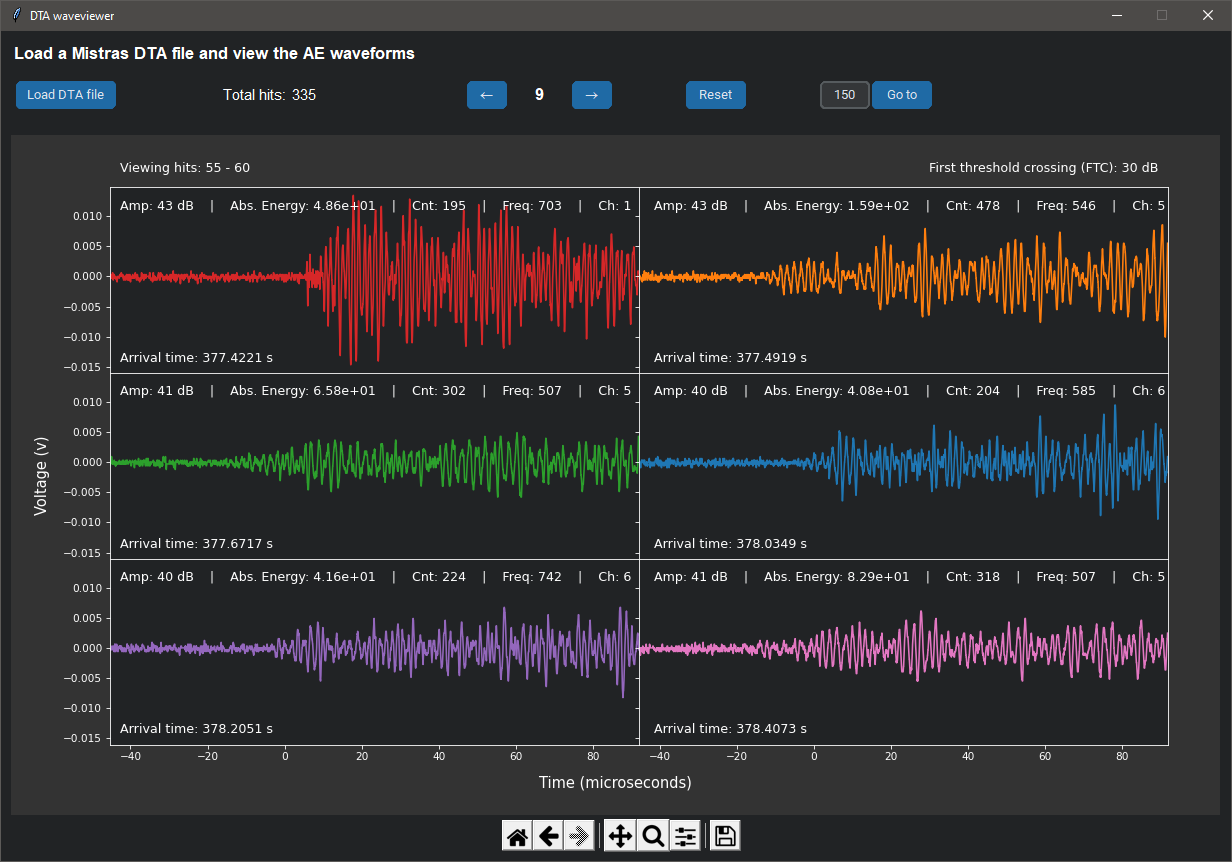
II. Interactive DTA waveviewer
For Acoustic Emissions detection experiments in the LVP, the Mistras/GMA acquisition software AEwin is used. Using this custom software, you can view your AE data directly by opening the proprietary file format *.dta. Like the above app 'DTA extract', the waveviewer apps also make use of MistrasDTA:
You can download both the python file and the compiled executable below:
If you only wish to see the waveforms that belong to events, you can use the modified app below. You also have the option to exclude a bad channel.
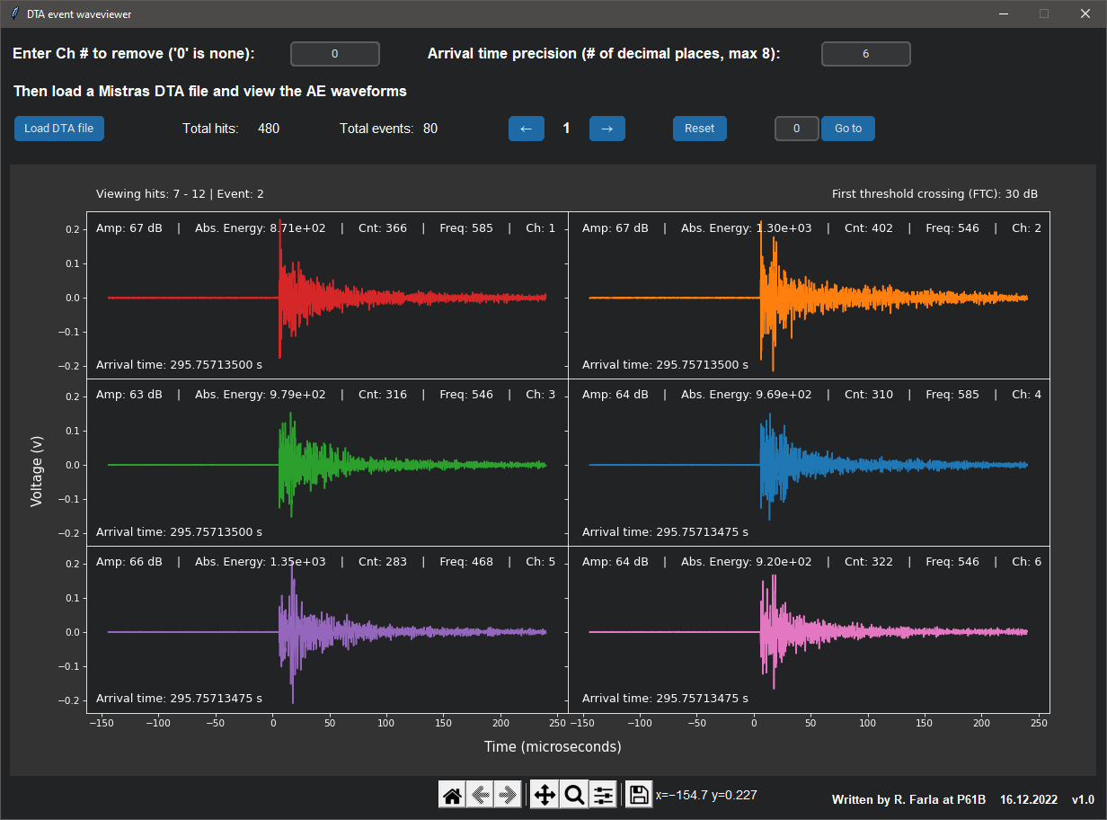
Version 1.1: Added a notification dialogue when no events can be found based on the chosen arrival time precision (python script only!)